This vignette demonstrates the complete rmaverick analysis pipeline, including:
- importing data
- running the main MCMC
- diagnosing good and bad MCMC behaviour
- comparing different models
- producing basic outputs
Simulate some data
rmverick comes with built-in functions for simulating data from different evolutionary models. The models used in simulation are exactly the same as the models used in the inference step, allowing us to test the power of the program without worrying about discrepancies between the data and the assumed model. We will simulate a data set of 100 diploid individuals, each genotyped at 20 loci and originating from 3 distinct subpopulations. We will assume no admixture between populations:
mysim <- sim_data(n = 100, loci = 20, K = 3, admix_on = FALSE)The simulated data takes the form of a list, and running names(mysim) we can see that it contains several elements:
names(mysim)## [1] "data" "allele_freqs" "admix_freqs" "group"The raw data is stored in the “data” element - this is the part that is equivalent to what we would see in real data. In addition, we have a record of the allele frequencies, admixture frequencies and grouping that were used in generating the data. These additional records can be useful in ground-truthing our estimated values later on, but are not actually used by the program, all that is needed for rmaverick analysis is the “data” element.
Data input into rmaverick must be in dataframe format. When using real data, any function that reads in a values in a dataframe can be used - for example the read.csv() and read.table() functions. Running head(mysim$data) we can see the general data format required by rmaverick:
head(mysim$data)## ID pop ploidy locus1 locus2 locus3 locus4 locus5 locus6 locus7 locus8
## 1 ind1 1 2 4 1 4 4 3 4 2 3
## 2 ind1 1 2 3 1 4 4 4 3 4 3
## 3 ind2 1 2 2 1 4 5 2 3 5 3
## 4 ind2 1 2 2 1 2 5 3 4 4 4
## 5 ind3 1 2 2 2 5 1 1 3 4 3
## 6 ind3 1 2 2 1 1 2 3 4 4 3
## locus9 locus10 locus11 locus12 locus13 locus14 locus15 locus16 locus17
## 1 5 2 3 4 2 4 4 3 2
## 2 5 1 5 5 3 5 4 3 4
## 3 1 2 5 3 5 3 5 1 4
## 4 1 1 3 1 3 4 5 3 2
## 5 2 2 2 3 2 2 5 3 5
## 6 3 1 5 5 3 1 4 2 5
## locus18 locus19 locus20
## 1 1 1 3
## 2 1 1 4
## 3 1 3 2
## 4 2 1 2
## 5 1 1 2
## 6 4 1 1Samples are in rows and loci are in columns, meaning for polyploid individuals multiple rows must be used for the same individual (here two rows per individual). There are also several meta-data columns, including the sample ID, the population of origin, and the ploidy. These meta-data columns are optional and can be turned on or off when loading the data into a project. Note that any ploidy level is supported by rmaverick, including mixed ploidy which can be specified using the ploidy column.
Data can also be arranged in wide format, with one row per sample and several columns per locus. If using this format there should be no ploidy column, as the ploidy is dictated by the number of columns per locus.
Create a project and read in data
rmaverick works with projects, which are essentially just lists containing all the inputs and outputs of a given analysis. We start by creating a project and loading in our data:
myproj <- mavproject()
myproj <- bind_data(myproj, df = mysim$data, ID_col = 1, pop_col = 2, ploidy_col = 3)
Alternatively, if you are familiar with the pipe operator %>% from the magrittr package (often imported via dplyr) then you can use this to chain together multiple commands:
library(dplyr)

myproj <- mavproject() %>%
  bind_data(df = mysim$data, ID_col = 1, pop_col = 2, ploidy_col = 3)
In the input arguments we have specified which columns are meta-data, and all other columns are assumed to contain genetic data. If using wide format data then the argument wide_format = TRUE should be used, and ploidy should be specified using the ploidy argument (mixed ploidy is not allowed in wide format).
We can view the project to check that the data have been loaded in correctly:
myproj## DATA:
## individuals = 100
## loci = 20
## ploidy = 2
## pops = 3
## missing data = 0 of 4000 gene copies (0%)
##
## PARAMETER SETS:
## (none defined)If there have been any mistakes in reading in the data, for example if meta-data columns have not been specified and so have been interpreted as genetic data (a common mistake), then this should be visible at this stage.
Define parameters and run basic MCMC
We can define different evolutionary models by using different parameter sets. Our first parameter set will represent a simple no-admixture model, i.e. the same model that was used to generate the data.
myproj <- new_set(myproj, name = "correct model (no admixture)", admix_on = FALSE)Producing a summary of the project we can now see additional properties, including the current active set and the parameters of this set.
myproj## DATA:
## individuals = 100
## loci = 20
## ploidy = 2
## pops = 3
## missing data = 0 of 4000 gene copies (0%)
##
## PARAMETER SETS:
## * SET1: correct model (no admixture)
##
## ACTIVE SET: SET1
## model = no-admixture
## lambda = 1Now we are ready to run a basic MCMC. We will start by exploring values of K from 1 to 5, using 1000 burn-in iterations and 1000 sampling iterations. By default the MCMC has auto_converge turned on, meaning it will test for convergence every convergence_test iterations and will exit if convergence is reached (convergence_test = burnin/10 by default). Hence, it is generally a good idea to set burnin to be higher than expected, as the MCMC will adjust this number down if needed. The number of sampling iterations can also be tuned. Our aim when choosing the number of sampling iterations should be to obtain enough samples that our posterior estimates are accurate to an acceptable tolerance level, but not so many that we waste time running the MCMC for long periods past this point. We will look into this parameter again once the MCMC has completed. The most unfamiliar parameter for most users will be the number of “rungs”. rmaverick runs multiple MCMC chains simultaneously, each at a different rung on a “temperature ladder”. The cold chain is our ordinary MCMC chain, and the hot chains serve two purposes: 1) they improve MCMC mixing, 2) they are central to the GTI method of estimating the evidence for different models. Finally, for the sake of this document we will run with pb_markdown = TRUE to avoid printing large amounts of output, but you should run without this argument.
myproj <- run_mcmc(myproj, K = 1:5, burnin = 1e3, samples = 1e3,
                   rungs = 10, pb_markdown =  TRUE)
## Calculating exact solution for K = 1
## completed in 0.00804694 seconds
##
## Running MCMC for K = 2
## Burn-in phase
##
|
|======================================================================| 100%
## converged within 300 iterations
## Sampling phase
##
|
|======================================================================| 100%
## completed in 3.40451 seconds
##
## Running MCMC for K = 3
## Burn-in phase
##
|
|======================================================================| 100%
## Warning: convergence still not reached within 1000 iterations
## Sampling phase
##
|
|======================================================================| 100%
## completed in 6.55462 seconds
##
## Running MCMC for K = 4
## Burn-in phase
##
|
|======================================================================| 100%
## converged within 400 iterations
## Sampling phase
##
|
|======================================================================| 100%
## completed in 5.32087 seconds
##
## Running MCMC for K = 5
## Burn-in phase
##
|
|======================================================================| 100%
## converged within 400 iterations
## Sampling phase
##
|
|======================================================================| 100%
## completed in 6.26428 seconds
##
## Processing results## Total run-time: 22.66 seconds##
## **WARNING** at least one MCMC run did not converge within specified burn-inNotice that the solution for K=1 is almost instantaneous, as no MCMC is required in this case. If any values of K failed to converge then we can use the same run_mcmc() function to re-run the MCMC for just a single value of K and with a longer maximum burn-in. This will overwrite the existing output for the specified value of K, but will leave all other values untouched:
myproj <- run_mcmc(myproj, K = 4:5, burnin = 1e4, converge_test = 100, samples = 1e3,
                   rungs = 10, pb_markdown =  TRUE)
## Running MCMC for K = 4
## Burn-in phase
##
|
|======================================================================| 100%
## converged within 1000 iterations
## Sampling phase
##
|
|======================================================================| 100%
## completed in 7.55933 seconds
##
## Running MCMC for K = 5
## Burn-in phase
##
|
|======================================================================| 100%
## converged within 900 iterations
## Sampling phase
##
|
|======================================================================| 100%
## completed in 8.43448 seconds
##
## Processing results## Total run-time: 17.08 secondsChecking MCMC performance
Before going any further with our analysis, it is critical that we check our MCMC performance. Without this stage we may end up reading into a particular set of results when in fact they are junk because the posterior has not been well explored. Fortunately, the temperature-based MCMC method inside rmaverick can help in producing reliable results as well as being used to estimate the evidence for a particular model. It does this by linking different heated chains together - the hotter chains explore a more diffuse version of the posterior and can then pass this information to the colder chains. We can check that information is being passed up and down the “rungs” of the temperature ladder by looking at the acceptance rate of these proposed moves, i.e. what proportion of swaps between adjacent rungs are accepted. This proportion needs to be non-zero for all pairs of rungs, otherwise information is not passing freely from the bottom of the ladder all the way to the top.
We can use the function plot_mc_acceptance() to explore the acceptance rate between all pairs of rungs:
plot_mc_acceptance(myproj, K = 2)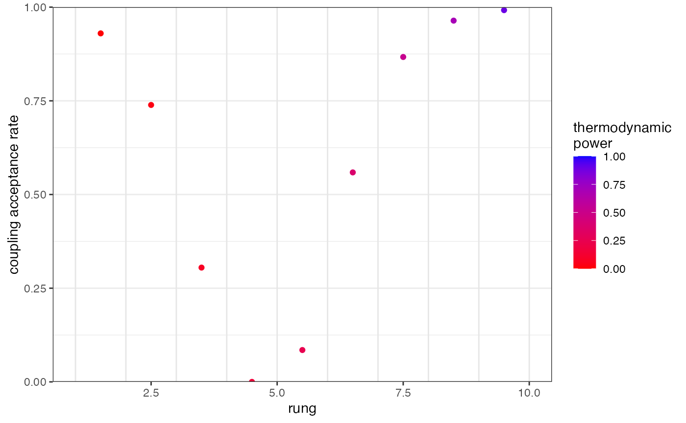
As a side note, all plots produced by rmaverick are produced using ggplot, meaning they can be stored and modified later on - for example adding titles, legends etc.
We can see that acceptance rates drop in the middle of our temperature ladder, meaning the hottest chains are unable to pass information up to the coldest chains. The simplest way to remedy this is to re-run with a larger number of temperature rungs. This check should be performed on every value of K:
myproj <- run_mcmc(myproj, K = 2:5, burnin = 1e4, converge_test = 100, samples = 1e3,
                   rungs = 50, pb_markdown =  TRUE)
## Running MCMC for K = 2
## Burn-in phase
##
|
|======================================================================| 100%
## converged within 300 iterations
## Sampling phase
##
|
|======================================================================| 100%
## completed in 15.3104 seconds
##
## Running MCMC for K = 3
## Burn-in phase
##
|
|======================================================================| 100%
## converged within 1100 iterations
## Sampling phase
##
|
|======================================================================| 100%
## completed in 30.9283 seconds
##
## Running MCMC for K = 4
## Burn-in phase
##
|
|======================================================================| 100%
## converged within 1200 iterations
## Sampling phase
##
|
|======================================================================| 100%
## completed in 39.0046 seconds
##
## Running MCMC for K = 5
## Burn-in phase
##
|
|======================================================================| 100%
## converged within 1900 iterations
## Sampling phase
##
|
|======================================================================| 100%
## completed in 60.8534 seconds
##
## Processing results## Total run-time: 2.46 minutesRepeating the plot we can see that acceptance rates are now acceptable:
plot_mc_acceptance(myproj, K = 2)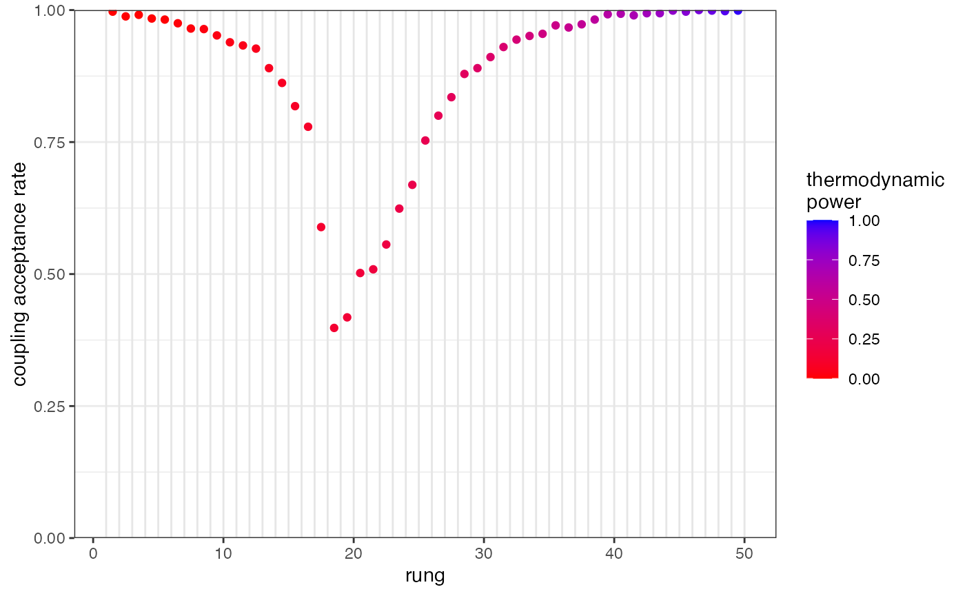
Run-time scales approximately linearly with the number of rungs, so adding more rungs like this can slow down the analysis quite considerably. However, this is the closest thing that you can get in the MCMC world to a guarantee that the full posterior has been explored. This is very important when there are multiple plausible ways of subdividing the population, and unfortunately we don’t know this without fully exploring the posterior distribution (a classic catch-22) hence the argument for using this method as standard.
There is another way to improve acceptance rates without increasing the number of rungs, and that is to change the distribution of rungs on the ladder. The parameter GTI_pow dictates how concentrated rungs are towards the left of the plot above. We can see this by re-plotting, but this time with the true thermodynamic power on the x-axis:
plot_mc_acceptance(myproj, K = 2, x_axis_type = 2)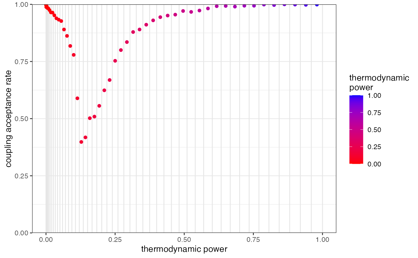
Concentrating rungs together increases the acceptance rate between them. This MCMC was run with GTI_pow=2, hence rungs are slightly squashed to the left, which will improve acceptance rates near 0 and will worsen acceptance rates near 1. If we were to re-run with a higher value we would see values even more concentrated near 0, which may have a slight beneficial effect in this case, although increasing the number of rungs has already done most of the heavy lifting in this example.
Comparing values of K
The GTI method estimates the evidence for a given model by combining information across the different temperature rungs. These rungs provide a series of point estimates that together make a “path”, and the final evidence estimate is computed from the area between this path and the zero-line. We can visualise this path using the plot_GTI_path() function:
plot_GTI_path(myproj, K = 3)
In order for our evidence estimate to be unbiased it is important that the GTI path is relatively smooth. As before, we can modify the smoothness of the path in two ways: 1) by increasing the number of rungs, 2) by changing the value of GTI_pow which controls the curvature of the path (higher values lead to more steep curvature). Ideally we want a straight path, i.e. we want as little curvature as possible. In the example above we have a good number of rungs and a nice straight path, so there is no need to re-run the MCMC. As with the acceptance rates analysis, this check should be performed on every value of K.
Once we are happy with our GTI paths we can look at our evidence estimates, first of all in log space:
plot_logevidence_K(myproj)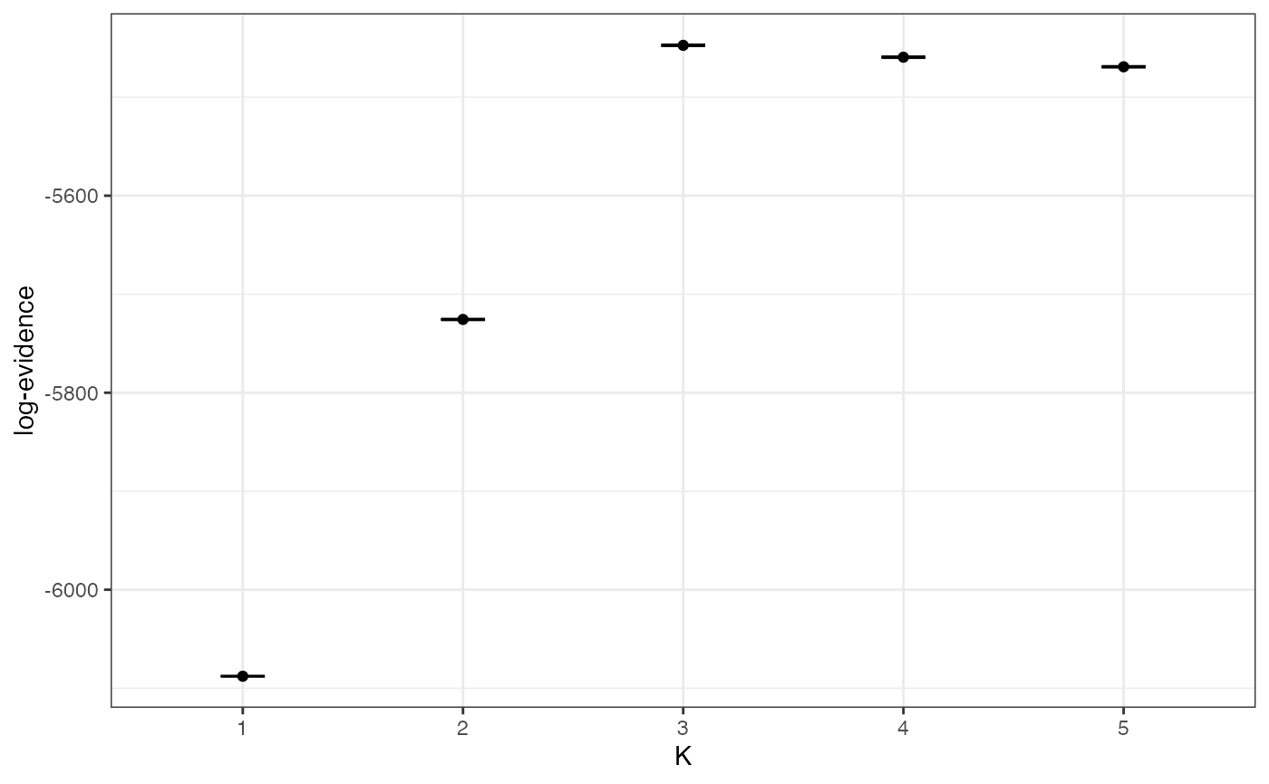
We can see a clear signal for K=3 or higher, and the 95% credible intervals are nice and tight. If we needed tighter credible intervals at this stage then we could re-run the MCMC (for the problem values of K only) with a larger number of samples.
We can also plot the full posterior distribution of K, which is obtained by transforming these values out of log space and normalising to sum to one:
plot_posterior_K(myproj)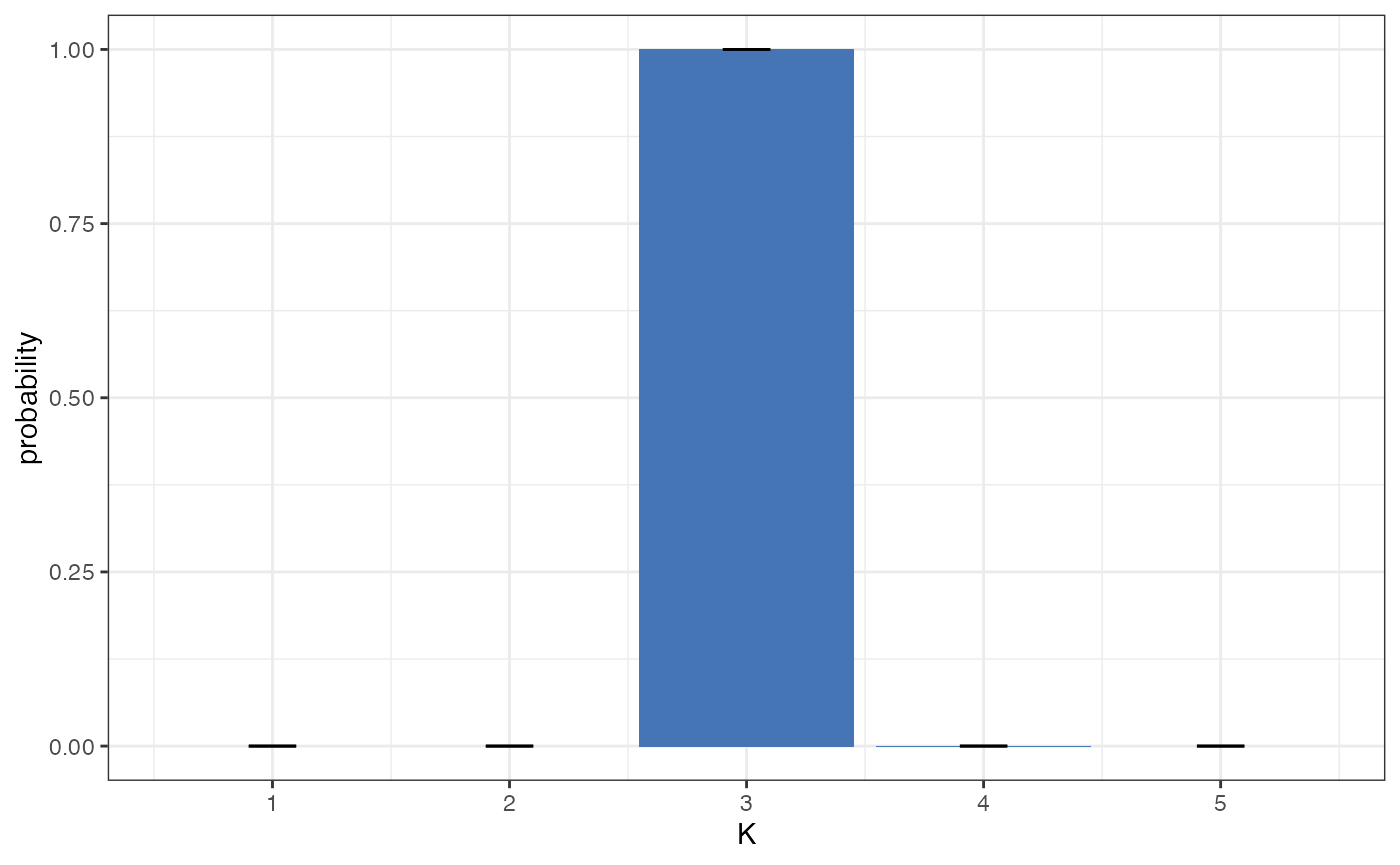
This second plot is usually more straightforward to interpret, as it is in linear space and so can be understood in terms of ordinary probability. In this example we can see strong evidence for K=3, with a posterior probability of >0.99. Again, if we had seen wide credible intervals at this stage then it would have been worth repeating the MCMC with a larger number of samples, but in this case the result is clear and so there is no need.
Structure plots
The main result of interest from this sort of analysis is usually the posterior allocation or “structure” plot. This plot contains one bar for each individual, with the proportion of each colour giving the posterior probability of belonging to each of the K subpopulations. We can use the plot_qmatrix() function to produce posterior allocation plots for different values of K. The divide_ind_on argument adds white lines between individuals, and can be turned off if these lines start getting in the way.
plot_qmatrix(myproj, K = 2:5, divide_ind_on = TRUE)
We can see that for K=3 (the most highly supported value of K) there is a clear split into three distinct subpopulations. The advantage of simulated data is that we can verify that this is the correct grouping by looking at mysim$group, although obviously this is not possible for real data.
When reporting and publishing results it is a good idea to produce posterior allocation plots for a range of values of K so that the reader has the option of visualising structure at multiple levels, and ideally this should also be backed up by a plot of the model evidence to give some idea of the model support at each level. At this stage it is worth stressing the point made by many previous authors - the model used by rmaverick and similar programs is just a cartoon of reality, and there is no strict K in the real world. Instead, each K captures a different level of population structure, and while the evidence can help guide us towards values of K that fit the data well, it is just a guide and should be taken alongside other biological considerations.
Admixture model
We will also run the simulated data through the admixture model, partly to explore how this model differs in implementation from the simpler no-admixture model, and partly to test whether rmaverick can detect that this model is inappropriate for the current data (recall that data were generated from the no-admixture model).
We start by creating a new parameter set, this time under the admixture model with the parameter alpha free to be estimated by the MCMC. Alpha controls the level of admixture, with larger values indicating a greater probability of inheriting genes from multiple subpopulations. We arrive back at the no-admixture model when alpha equals zero.
myproj <- new_set(myproj, name = "incorrect model (admixture)", admix_on = TRUE,
                  estimate_alpha = TRUE)
myproj
## DATA:
## individuals = 100
## loci = 20
## ploidy = 2
## pops = 3
## missing data = 0 of 4000 gene copies (0%)
##
## PARAMETER SETS:
## SET1: correct model (no admixture)
## * SET2: incorrect model (admixture)
##
## ACTIVE SET: SET2
## model = admixture
## estimate alpha = TRUE
## lambda = 1The admixture model tends to take considerably longer to run than the no-admixture model, and mixes more poorly. This is because the MCMC now has to consider the population assignment of each gene copy separately rather than moving all genes within an individual in a single block, and also the model has additional parameters to estimate. For this reason we suggest that if there is no prior biological reason to expect admixture between populations then consider running the simpler non-admixture model only.
We run the MCMC the same way as before, this time anticipating that we might need a greater number of burn-in and sampling iterations. Again, this should be run without the pb_markdown = TRUE argument ordinarily.
myproj <- run_mcmc(myproj, K = 1:5, burnin = 1e4, converge_test = 100, samples = 2e3,
                   rungs = 50, pb_markdown = FALSE)
## Calculating exact solution for K = 1
## completed in 1.13762 seconds
##
## Running MCMC for K = 2
## Burn-in phase
##
|
| | 0%
|
|= | 1%
|
|= | 2%
|
|== | 3%
|
|=== | 4%
|
|==== | 5%
|
|==== | 6%
|
|======================================================================| 100%
## converged within 700 iterations
## Sampling phase
##
|
| | 0%
|
|= | 1%
|
|= | 2%
|
|== | 3%
|
|=== | 4%
|
|==== | 5%
|
|==== | 6%
|
|===== | 7%
|
|====== | 8%
|
|====== | 9%
|
|======= | 10%
|
|======== | 11%
|
|======== | 12%
|
|========= | 13%
|
|========== | 14%
|
|=========== | 15%
|
|=========== | 16%
|
|============ | 17%
|
|============= | 18%
|
|============= | 19%
|
|============== | 20%
|
|=============== | 21%
|
|=============== | 22%
|
|================ | 23%
|
|================= | 24%
|
|================== | 25%
|
|================== | 26%
|
|=================== | 27%
|
|==================== | 28%
|
|==================== | 29%
|
|===================== | 30%
|
|====================== | 31%
|
|====================== | 32%
|
|======================= | 33%
|
|======================== | 34%
|
|========================= | 35%
|
|========================= | 36%
|
|========================== | 37%
|
|=========================== | 38%
|
|=========================== | 39%
|
|============================ | 40%
|
|============================= | 41%
|
|============================= | 42%
|
|============================== | 43%
|
|=============================== | 44%
|
|================================ | 45%
|
|================================ | 46%
|
|================================= | 47%
|
|================================== | 48%
|
|================================== | 49%
|
|=================================== | 50%
|
|==================================== | 51%
|
|==================================== | 52%
|
|===================================== | 53%
|
|====================================== | 54%
|
|======================================= | 55%
|
|======================================= | 56%
|
|======================================== | 57%
|
|========================================= | 58%
|
|========================================= | 59%
|
|========================================== | 60%
|
|=========================================== | 61%
|
|=========================================== | 62%
|
|============================================ | 63%
|
|============================================= | 64%
|
|============================================== | 65%
|
|============================================== | 66%
|
|=============================================== | 67%
|
|================================================ | 68%
|
|================================================ | 69%
|
|================================================= | 70%
|
|================================================== | 71%
|
|================================================== | 72%
|
|=================================================== | 73%
|
|==================================================== | 74%
|
|===================================================== | 75%
|
|===================================================== | 76%
|
|====================================================== | 77%
|
|======================================================= | 78%
|
|======================================================= | 79%
|
|======================================================== | 80%
|
|========================================================= | 81%
|
|========================================================= | 82%
|
|========================================================== | 83%
|
|=========================================================== | 84%
|
|============================================================ | 85%
|
|============================================================ | 86%
|
|============================================================= | 87%
|
|============================================================== | 88%
|
|============================================================== | 89%
|
|=============================================================== | 90%
|
|================================================================ | 91%
|
|================================================================ | 92%
|
|================================================================= | 93%
|
|================================================================== | 94%
|
|=================================================================== | 95%
|
|=================================================================== | 96%
|
|==================================================================== | 97%
|
|===================================================================== | 98%
|
|===================================================================== | 99%
|
|======================================================================| 100%
## completed in 189.285 seconds
##
## Running MCMC for K = 3
## Burn-in phase
##
|
| | 0%
|
|= | 1%
|
|= | 2%
|
|======================================================================| 100%
## converged within 300 iterations
## Sampling phase
##
|
| | 0%
|
|= | 1%
|
|= | 2%
|
|== | 3%
|
|=== | 4%
|
|==== | 5%
|
|==== | 6%
|
|===== | 7%
|
|====== | 8%
|
|====== | 9%
|
|======= | 10%
|
|======== | 11%
|
|======== | 12%
|
|========= | 13%
|
|========== | 14%
|
|=========== | 15%
|
|=========== | 16%
|
|============ | 17%
|
|============= | 18%
|
|============= | 19%
|
|============== | 20%
|
|=============== | 21%
|
|=============== | 22%
|
|================ | 23%
|
|================= | 24%
|
|================== | 25%
|
|================== | 26%
|
|=================== | 27%
|
|==================== | 28%
|
|==================== | 29%
|
|===================== | 30%
|
|====================== | 31%
|
|====================== | 32%
|
|======================= | 33%
|
|======================== | 34%
|
|========================= | 35%
|
|========================= | 36%
|
|========================== | 37%
|
|=========================== | 38%
|
|=========================== | 39%
|
|============================ | 40%
|
|============================= | 41%
|
|============================= | 42%
|
|============================== | 43%
|
|=============================== | 44%
|
|================================ | 45%
|
|================================ | 46%
|
|================================= | 47%
|
|================================== | 48%
|
|================================== | 49%
|
|=================================== | 50%
|
|==================================== | 51%
|
|==================================== | 52%
|
|===================================== | 53%
|
|====================================== | 54%
|
|======================================= | 55%
|
|======================================= | 56%
|
|======================================== | 57%
|
|========================================= | 58%
|
|========================================= | 59%
|
|========================================== | 60%
|
|=========================================== | 61%
|
|=========================================== | 62%
|
|============================================ | 63%
|
|============================================= | 64%
|
|============================================== | 65%
|
|============================================== | 66%
|
|=============================================== | 67%
|
|================================================ | 68%
|
|================================================ | 69%
|
|================================================= | 70%
|
|================================================== | 71%
|
|================================================== | 72%
|
|=================================================== | 73%
|
|==================================================== | 74%
|
|===================================================== | 75%
|
|===================================================== | 76%
|
|====================================================== | 77%
|
|======================================================= | 78%
|
|======================================================= | 79%
|
|======================================================== | 80%
|
|========================================================= | 81%
|
|========================================================= | 82%
|
|========================================================== | 83%
|
|=========================================================== | 84%
|
|============================================================ | 85%
|
|============================================================ | 86%
|
|============================================================= | 87%
|
|============================================================== | 88%
|
|============================================================== | 89%
|
|=============================================================== | 90%
|
|================================================================ | 91%
|
|================================================================ | 92%
|
|================================================================= | 93%
|
|================================================================== | 94%
|
|=================================================================== | 95%
|
|=================================================================== | 96%
|
|==================================================================== | 97%
|
|===================================================================== | 98%
|
|===================================================================== | 99%
|
|======================================================================| 100%
## completed in 171.004 seconds
##
## Running MCMC for K = 4
## Burn-in phase
##
|
| | 0%
|
|= | 1%
|
|= | 2%
|
|== | 3%
|
|=== | 4%
|
|==== | 5%
|
|======================================================================| 100%
## converged within 600 iterations
## Sampling phase
##
|
| | 0%
|
|= | 1%
|
|= | 2%
|
|== | 3%
|
|=== | 4%
|
|==== | 5%
|
|==== | 6%
|
|===== | 7%
|
|====== | 8%
|
|====== | 9%
|
|======= | 10%
|
|======== | 11%
|
|======== | 12%
|
|========= | 13%
|
|========== | 14%
|
|=========== | 15%
|
|=========== | 16%
|
|============ | 17%
|
|============= | 18%
|
|============= | 19%
|
|============== | 20%
|
|=============== | 21%
|
|=============== | 22%
|
|================ | 23%
|
|================= | 24%
|
|================== | 25%
|
|================== | 26%
|
|=================== | 27%
|
|==================== | 28%
|
|==================== | 29%
|
|===================== | 30%
|
|====================== | 31%
|
|====================== | 32%
|
|======================= | 33%
|
|======================== | 34%
|
|========================= | 35%
|
|========================= | 36%
|
|========================== | 37%
|
|=========================== | 38%
|
|=========================== | 39%
|
|============================ | 40%
|
|============================= | 41%
|
|============================= | 42%
|
|============================== | 43%
|
|=============================== | 44%
|
|================================ | 45%
|
|================================ | 46%
|
|================================= | 47%
|
|================================== | 48%
|
|================================== | 49%
|
|=================================== | 50%
|
|==================================== | 51%
|
|==================================== | 52%
|
|===================================== | 53%
|
|====================================== | 54%
|
|======================================= | 55%
|
|======================================= | 56%
|
|======================================== | 57%
|
|========================================= | 58%
|
|========================================= | 59%
|
|========================================== | 60%
|
|=========================================== | 61%
|
|=========================================== | 62%
|
|============================================ | 63%
|
|============================================= | 64%
|
|============================================== | 65%
|
|============================================== | 66%
|
|=============================================== | 67%
|
|================================================ | 68%
|
|================================================ | 69%
|
|================================================= | 70%
|
|================================================== | 71%
|
|================================================== | 72%
|
|=================================================== | 73%
|
|==================================================== | 74%
|
|===================================================== | 75%
|
|===================================================== | 76%
|
|====================================================== | 77%
|
|======================================================= | 78%
|
|======================================================= | 79%
|
|======================================================== | 80%
|
|========================================================= | 81%
|
|========================================================= | 82%
|
|========================================================== | 83%
|
|=========================================================== | 84%
|
|============================================================ | 85%
|
|============================================================ | 86%
|
|============================================================= | 87%
|
|============================================================== | 88%
|
|============================================================== | 89%
|
|=============================================================== | 90%
|
|================================================================ | 91%
|
|================================================================ | 92%
|
|================================================================= | 93%
|
|================================================================== | 94%
|
|=================================================================== | 95%
|
|=================================================================== | 96%
|
|==================================================================== | 97%
|
|===================================================================== | 98%
|
|===================================================================== | 99%
|
|======================================================================| 100%
## completed in 206.908 seconds
##
## Running MCMC for K = 5
## Burn-in phase
##
|
| | 0%
|
|= | 1%
|
|= | 2%
|
|== | 3%
|
|=== | 4%
|
|==== | 5%
|
|==== | 6%
|
|===== | 7%
|
|====== | 8%
|
|====== | 9%
|
|======= | 10%
|
|======== | 11%
|
|======== | 12%
|
|========= | 13%
|
|======================================================================| 100%
## converged within 1400 iterations
## Sampling phase
##
|
| | 0%
|
|= | 1%
|
|= | 2%
|
|== | 3%
|
|=== | 4%
|
|==== | 5%
|
|==== | 6%
|
|===== | 7%
|
|====== | 8%
|
|====== | 9%
|
|======= | 10%
|
|======== | 11%
|
|======== | 12%
|
|========= | 13%
|
|========== | 14%
|
|=========== | 15%
|
|=========== | 16%
|
|============ | 17%
|
|============= | 18%
|
|============= | 19%
|
|============== | 20%
|
|=============== | 21%
|
|=============== | 22%
|
|================ | 23%
|
|================= | 24%
|
|================== | 25%
|
|================== | 26%
|
|=================== | 27%
|
|==================== | 28%
|
|==================== | 29%
|
|===================== | 30%
|
|====================== | 31%
|
|====================== | 32%
|
|======================= | 33%
|
|======================== | 34%
|
|========================= | 35%
|
|========================= | 36%
|
|========================== | 37%
|
|=========================== | 38%
|
|=========================== | 39%
|
|============================ | 40%
|
|============================= | 41%
|
|============================= | 42%
|
|============================== | 43%
|
|=============================== | 44%
|
|================================ | 45%
|
|================================ | 46%
|
|================================= | 47%
|
|================================== | 48%
|
|================================== | 49%
|
|=================================== | 50%
|
|==================================== | 51%
|
|==================================== | 52%
|
|===================================== | 53%
|
|====================================== | 54%
|
|======================================= | 55%
|
|======================================= | 56%
|
|======================================== | 57%
|
|========================================= | 58%
|
|========================================= | 59%
|
|========================================== | 60%
|
|=========================================== | 61%
|
|=========================================== | 62%
|
|============================================ | 63%
|
|============================================= | 64%
|
|============================================== | 65%
|
|============================================== | 66%
|
|=============================================== | 67%
|
|================================================ | 68%
|
|================================================ | 69%
|
|================================================= | 70%
|
|================================================== | 71%
|
|================================================== | 72%
|
|=================================================== | 73%
|
|==================================================== | 74%
|
|===================================================== | 75%
|
|===================================================== | 76%
|
|====================================================== | 77%
|
|======================================================= | 78%
|
|======================================================= | 79%
|
|======================================================== | 80%
|
|========================================================= | 81%
|
|========================================================= | 82%
|
|========================================================== | 83%
|
|=========================================================== | 84%
|
|============================================================ | 85%
|
|============================================================ | 86%
|
|============================================================= | 87%
|
|============================================================== | 88%
|
|============================================================== | 89%
|
|=============================================================== | 90%
|
|================================================================ | 91%
|
|================================================================ | 92%
|
|================================================================= | 93%
|
|================================================================== | 94%
|
|=================================================================== | 95%
|
|=================================================================== | 96%
|
|==================================================================== | 97%
|
|===================================================================== | 98%
|
|===================================================================== | 99%
|
|======================================================================| 100%
## completed in 292.948 seconds
##
## Processing results## Total run-time: 14.38 minutesAs before, we need to check the behaviour of our MCMC, starting with acceptance rates between rungs. This should be done for all values of K:
plot_mc_acceptance(myproj, K = 2)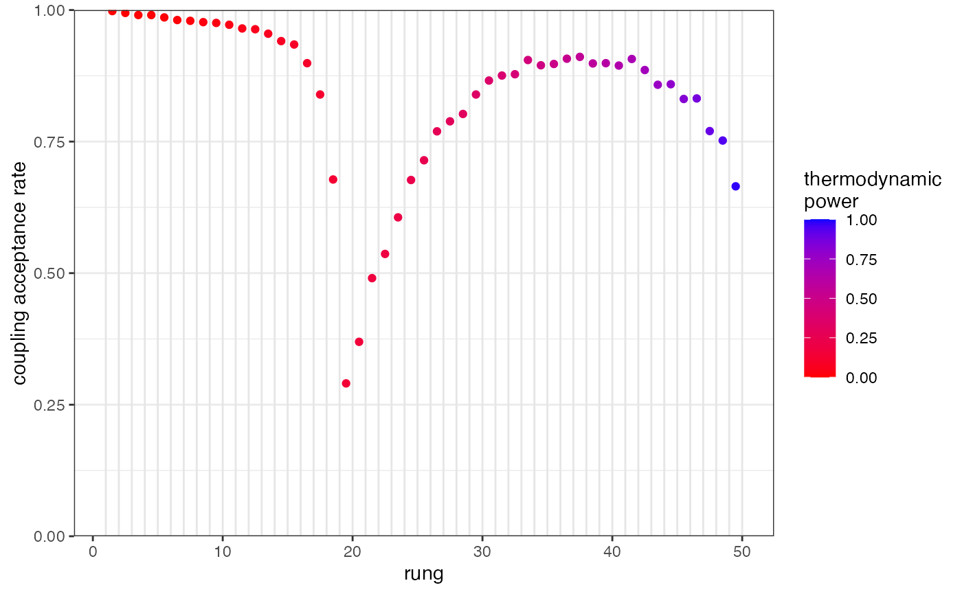
Under the admixture model we have the additional parameter alpha to check. We can produce a summary plot of this parameter as follows:
plot_alpha(myproj, K = 3)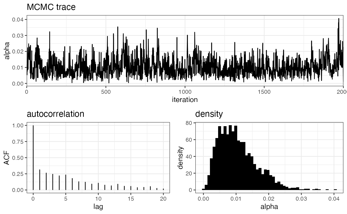
The MCMC trace shows the actual value of alpha at each iteration of the MCMC, the autocorrelation plot shows how far apart draws need to be before they are approximately independent (here ~40 draws), and the density plot gives the posterior distribution of alpha. Notice that the estimated value of alpha is very small (~0.01). This is an early indication that the no-admixture model may be more appropriate here, as the admixture model is essentially converging on this simpler model.
As before, we need to check that our GTI path is smooth and straight. Do this for all values of K:
plot_GTI_path(myproj, K = 3)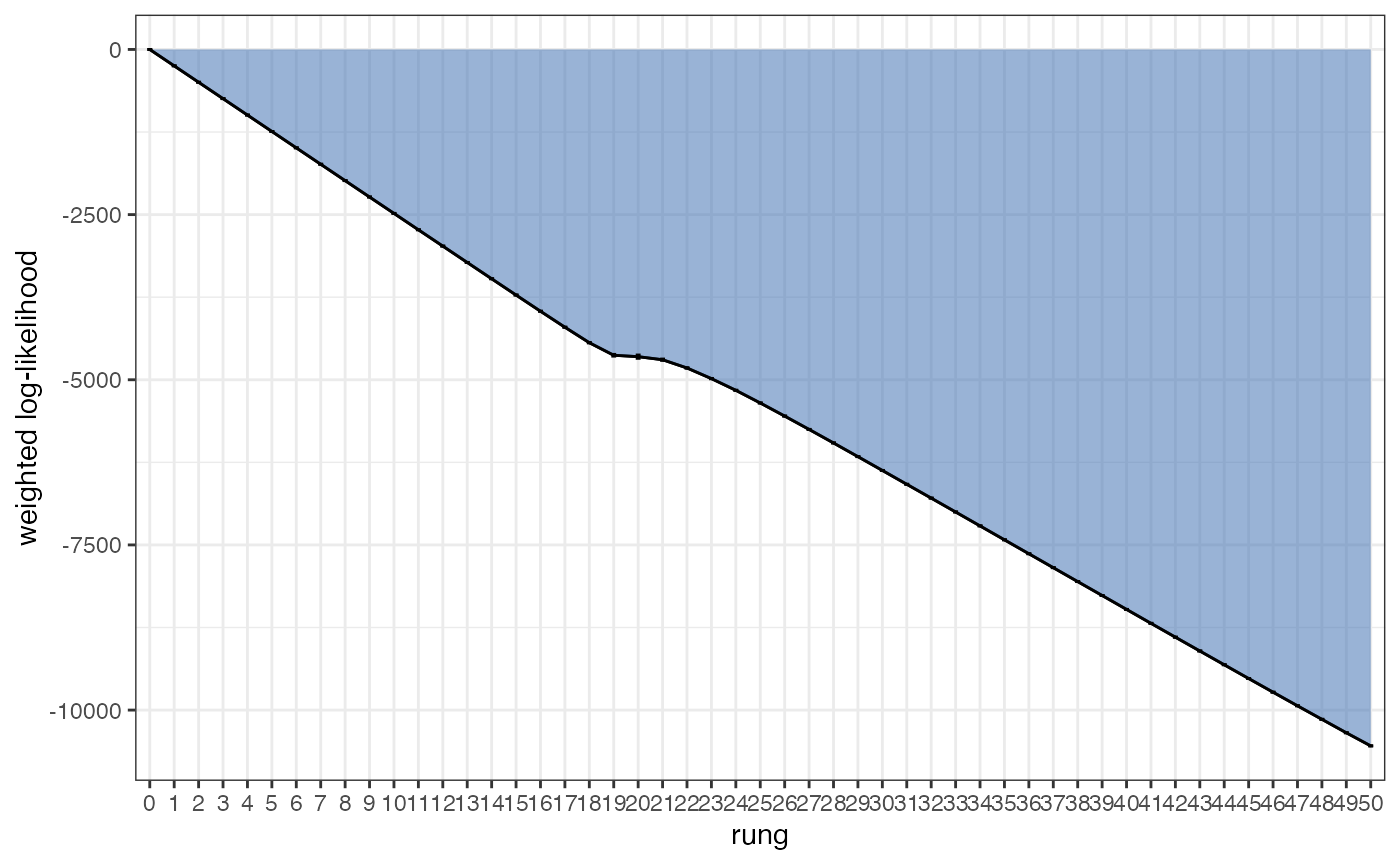
Assuming we are happy with these paths, we can visualise the evidence for each value of K in log space and linear space:
plot_logevidence_K(myproj)
plot_posterior_K(myproj)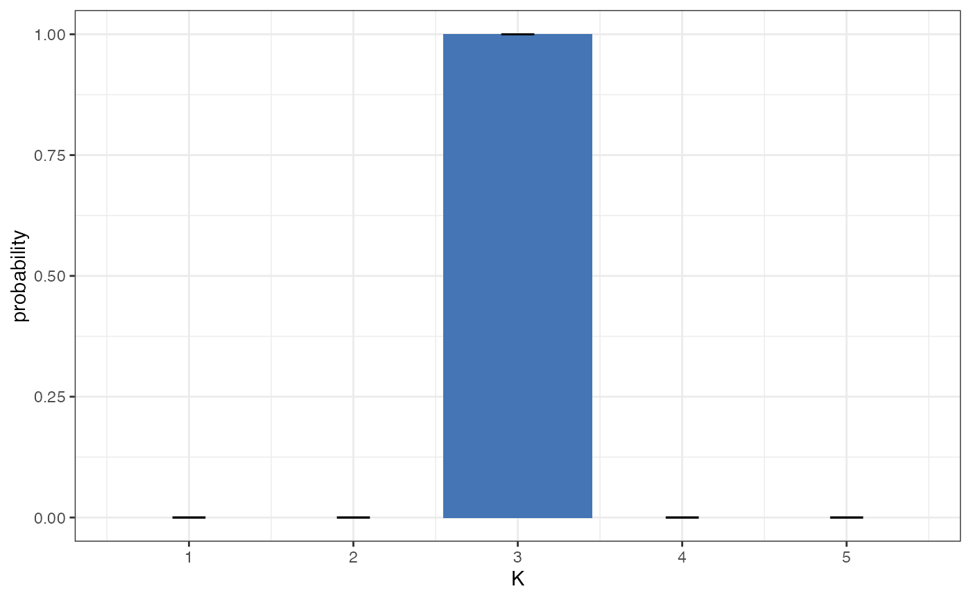
Again, there is clear evidence for K=3 under this model, despite the fact that this model is technically not appropriate for the simulated data.
Producing posterior allocation plots for a range of values of K we see results similar to the no-admixture model, with most individuals assigned to just a single subpopulation.
plot_qmatrix(myproj, K = 2:5, divide_ind_on = TRUE)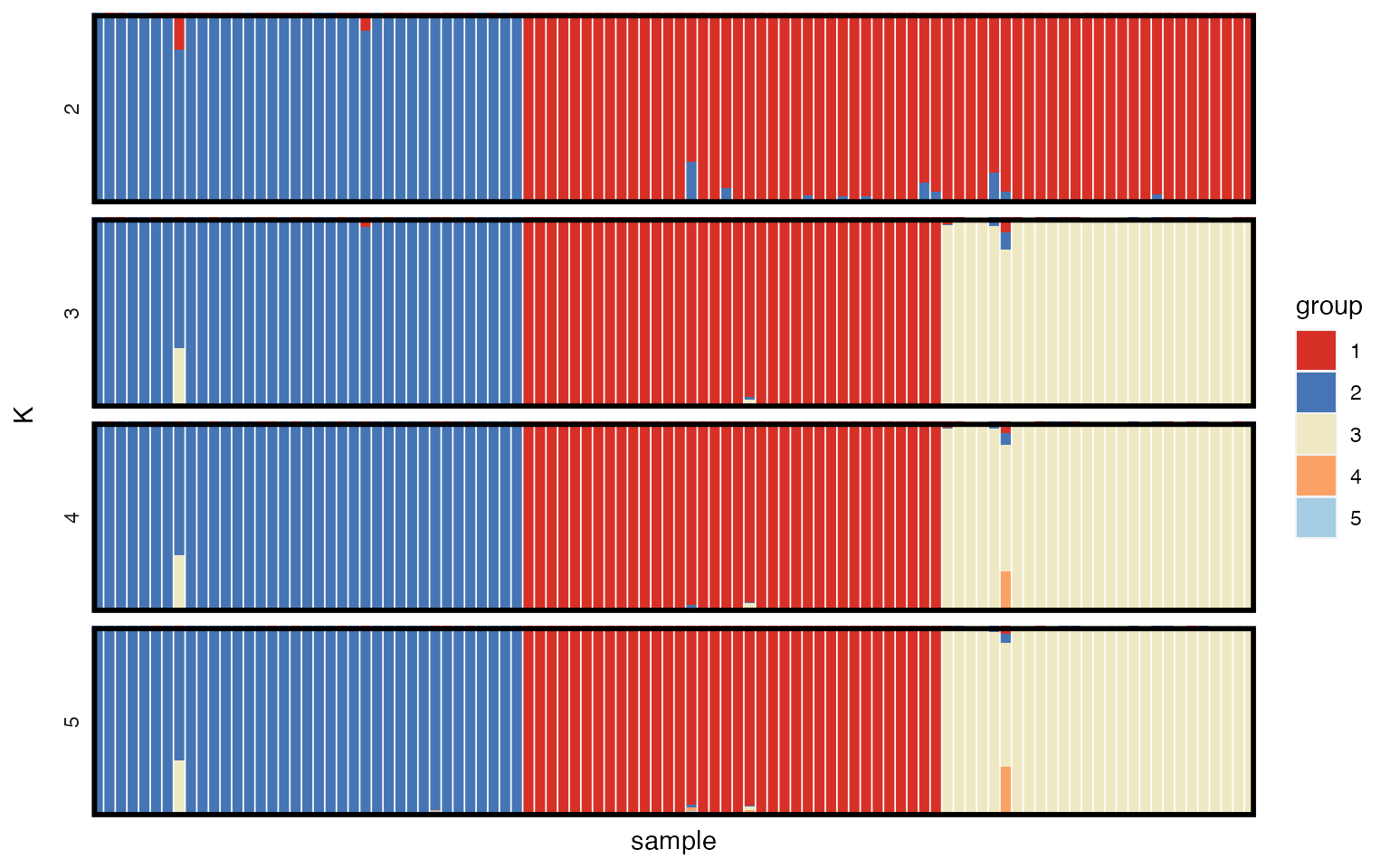
Comparing evolutionary models
Finally, we can make use of one of the major advantages of the model evidence - the ability to compare between different evolutionary models. The overall evidence of a model is taken as the average over all values of K under that model. We can plot the overall model evidence in log space using the plot_logevidence_model() function, and in the form of a posterior distribution using the plot_posterior_model() function:
plot_logevidence_model(myproj)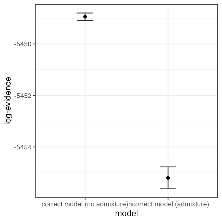
plot_posterior_model(myproj)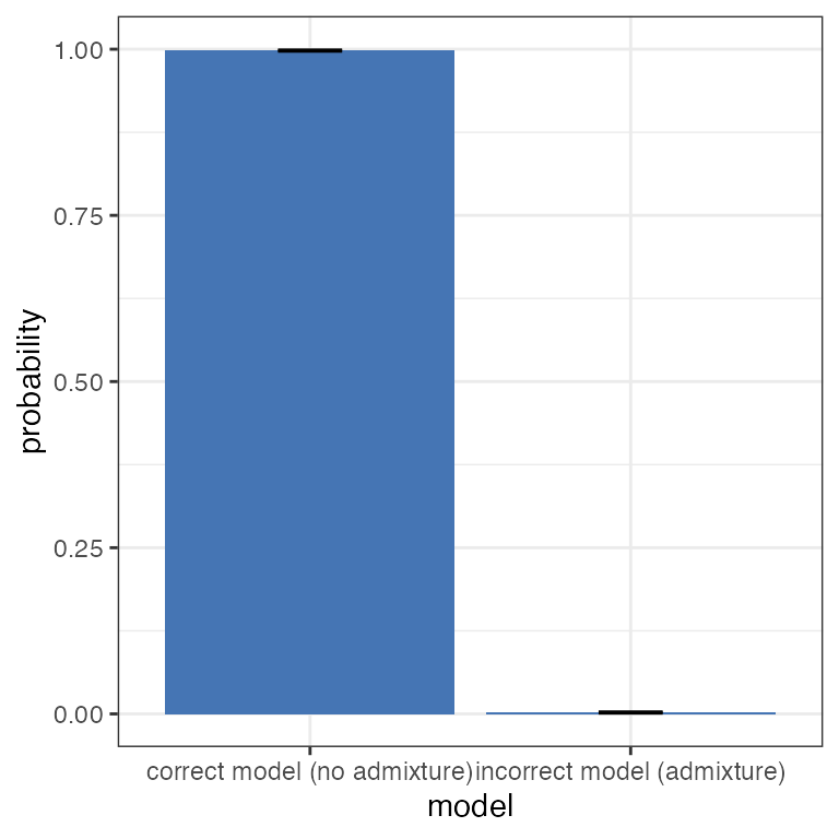
It is clear from these plots that there is far greater support for the no-admixture model, therefore we would be perfectly justified in ignoring the output from the admixture model and only reporting results of the no-admixture model. In other words, the data suggests that whatever admixture is present is minimal, which should be taken alongside other biological considerations.
At this point our basic analysis is complete. See this vignette on how to speed up the analysis by running in parallel over multiple cores.